Capacity Planning for Retrieval: A Practical Guide for RAG and Agent Memory Builders
Capacity planning for retrieval is a problem most guides don't acknowledge. The standard advice is written for agencies running web servers and IT teams managing VM pools. You're building something different: a vector index that must fit in RAM, embeddings that consume storage per dimension, queries that hit the database hundreds of times per second, and agent memory that competes with the context window for every token. Generic formulas won't help you. The honest answer is that retrieval capacity planning needs its own math, and GigaRAG was built for builders facing exactly these constraints. This guide covers the formulas you need: vector index sizing, embedding storage estimates, RAM requirements for in-memory versus disk-based indexes, query throughput budgets, and agent memory limits. It also tells you plainly what capacity planning cannot fix.
| At a glance | Details |
|---|---|
| Focus | Retrieval-specific capacity planning, not generic IT planning |
| Core formula | Index size = vectors × dimensions × bytes per value |
| Key levers | Vector count, dimensions, precision, index type |
| Throughput driver | Query rate, top-k, concurrency, latency budget |
| Agent memory | Budget tokens and retrieval calls per turn |
| Main risk | Under-provisioning RAM causes latency spikes and OOM |
In This Guide
- What Is Capacity Planning for Retrieval?
- In-Memory vs Disk-Based Vector Index: Capacity Trade-Offs
- The Three Classic Capacity Planning Strategies (Lead, Lag, Match)
- Capacity Planning For Retrieval: A Step-by-Step Guide
- How to Calculate Vector Index Size
- Estimating RAM and Memory Requirements
- Planning Query Throughput and Latency Budgets
- Agent Memory Budgets: A Retrieval-Specific Constraint
- Single-Node vs. Distributed Retrieval: Capacity Tradeoffs
- What Capacity Planning Cannot Do
- A Practical Capacity Planning Process for Retrieval
- Common Mistakes in Retrieval Capacity Planning
What Is Capacity Planning for Retrieval?
Capacity planning for retrieval is the process of estimating how much index storage, RAM, query throughput, and latency headroom your retrieval system needs before you deploy it, so you don't overpay or fall over under load.
Generic capacity planning asks how many servers or staff hours you need. Retrieval capacity planning asks different questions: how many vectors fit in your index, how much RAM that index consumes, how many queries per second it can serve, and how fast it returns results.
How retrieval capacity differs from generic capacity planning
A retail chain plans capacity in storefronts and warehouse shelves. A retrieval builder plans in vectors, dimensions, and milliseconds. The unit of work isn't a customer transaction. It's an embedding lookup against a high-dimensional index. That changes the math entirely.
The four capacity dimensions: index size, memory, throughput, latency
Four numbers matter. Index size is how much disk or RAM your vectors occupy. Memory is what the index needs resident to serve queries fast. Throughput is queries per second under load. Latency is the time from query to result, usually measured at p95 or p99. You can't tune one without affecting the others.
[!note] Capacity planning cannot fix poor retrieval quality — if recall is low due to bad chunking or embeddings, more RAM or QPS will not improve results. It also cannot predict sudden traffic spikes or data growth without accurate inputs.
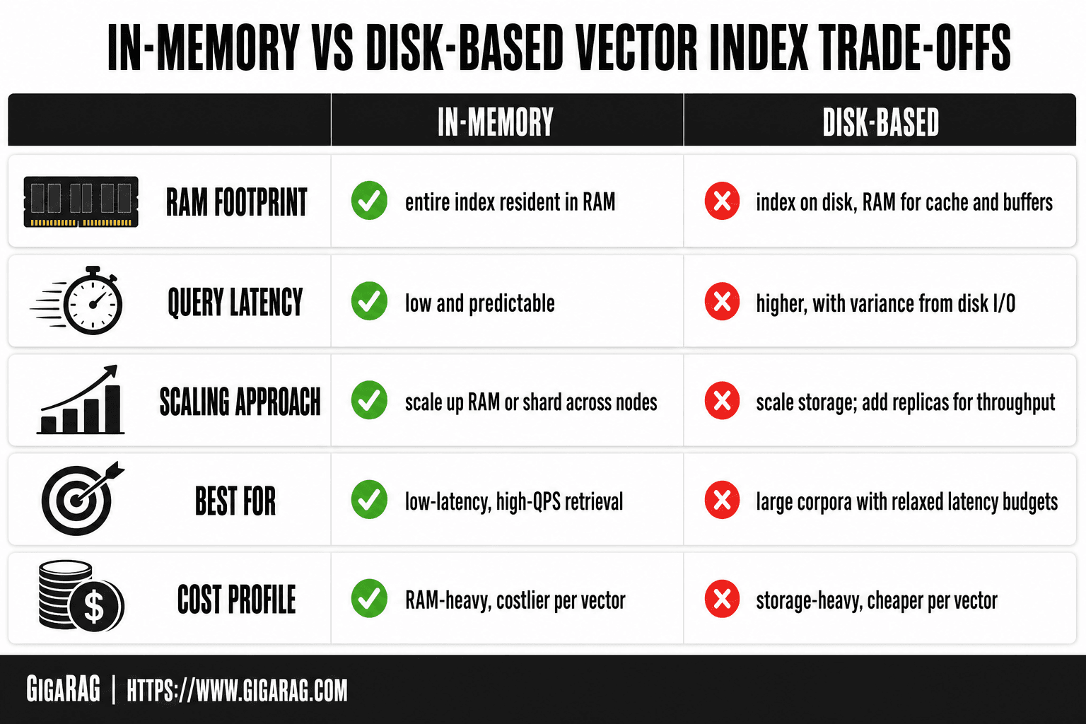
In-Memory vs Disk-Based Vector Index: Capacity Trade-Offs
| Factor | In-Memory Index | Disk-Based Index |
|---|---|---|
| RAM footprint | High — entire index resident in RAM | Lower — index on disk, RAM for cache and buffers |
| Query latency | Low and predictable | Higher, with variance from disk I/O |
| Scaling approach | Scale up RAM or shard across nodes | Scale storage; add replicas for throughput |
| Best for | Low-latency, high-QPS retrieval | Large corpora with relaxed latency budgets |
| Cost profile | RAM-heavy, costlier per vector | Storage-heavy, cheaper per vector |
The Three Classic Capacity Planning Strategies (Lead, Lag, Match)
Capacity planning strategies tell you when to add capacity relative to demand. Lead means you provision ahead of growth. Lag means you wait until you hit a limit, then scale. Match means you track demand closely and add capacity in small increments.
Lead strategy: pre-provisioning for anticipated index growth
Lead works when growth is predictable. You know a new customer is onboarding next quarter, or your embedding pipeline will ingest 2 million new vectors. You buy the RAM and storage before you need it. The cost is carrying unused capacity now. For retrieval, lead makes sense when index growth is contractual, not speculative.
Lag strategy: scaling after hitting memory or latency limits
Lag is reactive. You run until p95 latency crosses your budget or the index no longer fits in RAM, then you add nodes or move to disk. It's cheap until it isn't. Lag suits early-stage systems where traffic is unknown and over-provisioning would waste budget.
Match strategy: monitoring QPS and scaling incrementally
Match tracks QPS and index size continuously, adding capacity in small steps as demand rises. It requires monitoring and automation. For retrieval, match is the default once you have steady traffic: watch p95 latency and memory headroom, scale when either crosses a threshold you set.
[!tip] For agent memory systems, budget retrieval calls per turn and cache frequent queries — this often reduces required QPS more than adding nodes. Track tokens and calls per turn to keep memory budgets predictable.
Capacity Planning For Retrieval: A Step-by-Step Guide
- Estimate vector count: documents × average chunks per document.
- Choose embedding dimensions and precision (e.g., 768 or 1536 dims; float32 or int8).
- Compute raw vector size: vectors × dimensions × bytes per value.
- Add index overhead (graph links, metadata, payloads) as a multiplier.
- Set a query latency budget and derive required QPS per node from concurrency.
- Add headroom (e.g., 30–50%) for growth, replicas, and peak load.
- Validate with a load test using representative queries and top-k values.
How to Calculate Vector Index Size
The formula is simple. The hard part is knowing your numbers.
The core formula: vectors × dimensions × bytes per dimension
Index size = number of vectors × dimensions per vector × bytes per dimension.
That's it. A float32 vector uses 4 bytes per dimension. A float16 uses 2 bytes. An int8 quantized vector uses 1 byte. Binary vectors use 1 bit per dimension, or 0.125 bytes.
So a 1536-dimension embedding stored as float32 costs 6,144 bytes per vector. Store 1 million of those and you're at 6.14 GB before any index overhead.
Keep in mind: this is the raw vector data only. HNSW graphs add link structures on top, typically 10-30% overhead. Metadata, IDs, and payloads add more. Budget for it.
Worked example: 1M vectors at 1536 dimensions
Start with the raw math: 1,000,000 vectors × 1,536 dimensions × 4 bytes = 6.14 GB.
Add HNSW overhead at roughly 20%: 7.37 GB. Add metadata (say 200 bytes per record): another 200 MB. Total: around 7.6 GB for the index.
If you're running this in-memory, you need at least 8 GB of RAM just for the index, plus headroom for the OS and query processing. A 16 GB instance is the practical floor.
How quantization (int8, binary) reduces index size
Quantization shrinks each dimension. int8 cuts the 6.14 GB example to 1.54 GB. Binary cuts it to 192 MB. The tradeoff is recall: int8 typically loses 1-3% recall versus float32. Binary loses more, often 5-10% depending on your data.
The honest answer is: test before you commit. Run your actual queries against a quantized index and measure recall. If the drop is acceptable, the RAM savings are real. If not, stay at float32 and provision accordingly.
Estimating RAM and Memory Requirements
The index size math gets you the storage number. RAM is a different question, and the answer depends on where your index lives.
In-memory indexes: RAM = index size + overhead
HNSW and other graph-based indexes need the whole structure in RAM. Take the 7.6 GB index from the previous section. You need that much RAM, plus 20-30% headroom for query processing and OS overhead. A 16 GB instance is the floor, not the ceiling.
Disk-based indexes: RAM for cache and metadata only
IVF and DiskANN keep vectors on disk and load only what's needed. RAM holds the index metadata, the cache, and recently accessed vectors. A 100 GB disk index might need only 8-16 GB of RAM. The tradeoff is latency: disk reads are slower than memory reads, so p95 and p99 latency climb.
When to choose in-memory vs. disk-based
Choose in-memory when latency is the hard constraint and your index fits in affordable RAM. Choose disk-based when the index outgrows RAM or cost per GB matters more than a few milliseconds. Most RAG pipelines start in-memory and move to disk-based when the index passes 50-100 GB.
Planning Query Throughput and Latency Budgets
RAM gets you running. Throughput and latency decide whether users wait or leave.
Estimating QPS from user traffic and agent call patterns
Start with active users, not total users. If 10,000 daily active users each trigger 5 retrievals per session, that's 50,000 queries per day. Spread across an 8-hour peak window, you're looking at roughly 1.7 QPS average. Peak is what matters: multiply by 3-5x for burst traffic.
Agent call patterns change the math. A single user prompt can trigger 10-20 retrieval calls as the agent loops through tool use. One "active user" isn't one query. It's a fan-out.
Setting latency budgets: p50 vs. p95 vs. p99
p50 tells you the typical experience. p95 and p99 tell you the worst experience most users will actually hit. Set your budget at p95, not p50. A 50 ms p50 with a 400 ms p95 means 5% of users wait 8x longer.
For RAG, aim for p95 under 200 ms end-to-end. That includes embedding generation, index search, and reranking. Tight budgets force in-memory indexes. Loose budgets let you use disk.
How index type and hardware affect throughput
HNSW on a single node with 16 GB RAM handles 500-1,000 QPS at 1536 dimensions before latency degrades. Disk-based indexes drop that to 100-300 QPS but scale to far larger indexes. More CPU cores help throughput linearly until memory bandwidth becomes the bottleneck. Test with your actual embedding model. Benchmarks from other models don't transfer.
Agent Memory Budgets: A Retrieval-Specific Constraint
Retrieval capacity and agent memory are two sides of the same coin. You can size an index perfectly and still blow the agent's context window on the first call.
Context window limits and token budgets
An agent's context window is a hard ceiling. GPT-4-class models run 128k tokens, but usable space shrinks fast once system prompts, tool definitions, and conversation history take their cut. Budget 20-30% of the window for retrieved content. That's your retrieval ceiling, and it's smaller than you think.
How retrieved chunk size affects memory usage
Chunk size sets the floor for memory consumption. A 512-token chunk retrieved 10 times eats 5,120 tokens, whether the agent needs all of it or not. Smaller chunks give finer control but force more retrieval calls. Each call adds overhead: embedding time, index search, and the tokens spent on tool-use scaffolding.
Balancing retrieval depth with agent memory constraints
The honest answer is that retrieval depth and memory budget trade off directly. Top-k of 20 at 512 tokens per chunk is 10,240 tokens, roughly 8% of a 128k window. Push top-k to 50 and you're at 25,600 tokens, 20%. The fix is reranking: retrieve wide, then pass only the top 3-5 chunks into the agent. You get recall without the memory hit.
Single-Node vs. Distributed Retrieval: Capacity Tradeoffs
A single node handles more than most builders expect. A 1M-vector index at 1536 dimensions in float32 is roughly 6GB, which fits in RAM on a mid-range cloud instance. If your QPS stays under a few hundred and your index stays under a few million vectors, one node is enough. Don't shard prematurely.
When a single node is sufficient
The honest answer is it depends on two numbers: index size and QPS. If both fit comfortably on one machine with 50% headroom, stop there. Distributed systems add network hops, coordination overhead, and operational complexity. You pay that cost whether you need it or not.
Sharding: splitting the index across nodes
Sharding becomes necessary when the index outgrows one machine's RAM. You split vectors across nodes by ID range or hash. Each shard holds a slice of the index and answers queries independently, then results merge. Capacity math changes: total RAM is shard count times per-shard RAM, but query latency climbs because every query hits every shard.
Replication: duplicating for throughput and availability
Replication copies the same shard to multiple nodes. It doesn't increase capacity, it increases throughput and fault tolerance. Three replicas can serve three times the read QPS, but you pay three times the storage. Replication also buys you failover: lose one replica, queries keep flowing. The main catch is write amplification. Every vector insert must propagate to every replica, which slows ingestion as replica count grows.
What Capacity Planning Cannot Do
Capacity planning tells you how much hardware you need. It doesn't tell you whether your retrieval is any good. You can provision a perfect 6GB index and still ship a system that returns irrelevant chunks. The math works. The product doesn't.
Capacity planning cannot fix poor retrieval quality
If your embeddings are bad, more RAM won't save you. A 10M-vector index of poorly embedded documents returns 10M poorly matched results, just faster. The same goes for chunking. Split documents at arbitrary 500-token boundaries and you'll get fragments that don't answer anything. Capacity planning assumes your retrieval pipeline already works. It sizes the box, not the contents.
Capacity planning cannot predict black-swan traffic spikes
You can forecast growth from historical data. You cannot forecast a Hacker News front-page hit or a viral tweet. Those spikes arrive in minutes and multiply QPS by 10 or 100. Capacity planning handles trend growth, not step functions. For spikes, you need autoscaling, caching, or rate limiting, not a better spreadsheet.
Capacity planning cannot replace monitoring and alerting
A plan is a snapshot. Reality drifts. Indexes grow faster than forecast. Query patterns shift. Embedding models get swapped for larger ones. Without monitoring, you'll discover the gap when latency spikes or the node runs out of RAM at 3am. Monitoring tells you when the plan is wrong. Capacity planning just gives you a starting point.
A Practical Capacity Planning Process for Retrieval
You don't need a 40-page plan. You need five steps you can run in an afternoon, then revisit monthly.
Step 1: Measure current index size and QPS
Pull your vector count, dimensionality, and bytes per dimension from the database. Log QPS at peak, not average. Peak is what kills you.
Step 2: Forecast vector growth and query growth
Track weekly vector growth for a month, then extrapolate. For queries, use a moving average over 30 days. If growth is lumpy, forecast in ranges: low, expected, high.
Step 3: Calculate required RAM and storage
Multiply forecasted vectors by bytes per vector. Add 20% for index overhead. That's your RAM floor for in-memory. For disk-based, budget cache plus metadata.
Step 4: Provision with headroom
Provision for the high forecast, not the expected one. Headroom buys you time to react. 30% over expected is a reasonable starting point.
Step 5: Monitor and adjust
Set alerts on RAM usage, QPS, and p95 latency. When actuals drift from forecast by more than 20%, rerun the plan. Capacity planning is a loop, not a document.
Common Mistakes in Retrieval Capacity Planning
Most capacity failures come from four errors, and they're all avoidable.
Underestimating vector growth rate
Builders size for today's vector count, not next quarter's. If you add 50,000 vectors a week, that's 2.6 million a year. Plan for the slope, not the point.
Ignoring quantization as a cost-saving lever
int8 quantization cuts index size by 4x with a small recall hit. Skipping it means paying for RAM you don't need. Test recall before you commit, but don't dismiss it.
Forgetting agent memory constraints
An agent can only use what fits in its context window. Retrieving 20 chunks of 500 tokens each burns 10,000 tokens before the model thinks. Retrieval capacity and memory capacity are one budget.
Over-provisioning without monitoring data
Buying headroom you can't justify is waste. Provision for the high forecast, then let monitoring tell you when to scale. Capacity planning for retrieval is a loop, not a purchase order.
Frequently Asked Questions
What do you understand by capacity planning?
Capacity planning is the process of estimating the resources needed to meet current and future demand. For retrieval systems, it means sizing vector indexes, RAM, storage, and query throughput so latency and availability targets are met without over-provisioning.
What is the difference between MRP and CRP in operations management?
MRP (Material Requirements Planning) plans materials and components needed for production, while CRP (Capacity Requirements Planning) checks whether available capacity can meet the production plan. In retrieval, the analogous split is planning data/index size (materials) versus planning query throughput and compute (capacity).
What are those forecasting techniques for capacity planning?
Common techniques include trend analysis, moving averages, exponential smoothing, and scenario-based modeling. For retrieval, forecast vector growth from document ingestion rates and query growth from user or agent activity, then add headroom.
How do I calculate vector index size for RAG?
Start with vectors × dimensions × bytes per value (e.g., 4 bytes for float32, 1 byte for int8). Then multiply by an overhead factor for index structures and metadata. This gives a baseline RAM or storage estimate before headroom.
How many queries per second can one node handle?
It depends on index type, vector dimensions, top-k, and hardware. Measure with a load test using your actual data and query patterns. As a rule of thumb, in-memory indexes handle higher QPS than disk-based ones, but always validate.
What are the 7 types of planning?
In general management, common planning types include strategic, tactical, operational, contingency, financial, resource, and project planning. For retrieval capacity, the most relevant are operational (day-to-day throughput) and contingency (failover and peak load) planning.
How do I plan agent memory capacity?
Budget tokens and retrieval calls per agent turn, then multiply by expected concurrent agents. Cache frequent retrievals and summarize long contexts to reduce load. Monitor actual usage and adjust headroom as agent behavior evolves.
About GigaRAG
GigaRAG is for agent memory and RAG pipeline builders. get this right. Whether you are working through capacity planning for retrieval or something adjacent, we publish what we have actually tested, including where it falls short.